Smoothing Splines in R: A Tutorial

Nonparametric regression is an excellent descriptive tool that does not assume linearity; only assumes smoothness

21.1 Prominent people

Grace Wahba The International Prize in Statistics Foundation has awarded Grace Wahba the 2025 prize in recognition of her groundbreaking work on smoothing splines, which has transformed modern data analysis and machine learning.

21.2 Kernel regression

Uses weighted averages of nearby points to estimate the relationship

21.3 Smoothing splines

21.4 Introduction to Smoothing Splines

Smoothing splines are nonparametric regression techniques that fit flexible curves to data while controlling smoothness. They’re particularly useful when you want to model complex relationships without making strong assumptions about the functional form.

library(ggplot2)
library(mgcv)      # For GAMs, which include smoothing splines
library(splines)   # Basic spline functions

21.5 Basic Smoothing Spline Example

Let’s start with a simple example using simulated data with a non-linear pattern:

# Create some sample data with non-linear pattern
set.seed(123)
n <- 100
x <- sort(runif(n, 0, 10))
y <- sin(x) + 0.3*x + rnorm(n, 0, 0.3)
data <- data.frame(x = x, y = y)

# Fit smoothing spline using base R
spline_fit <- smooth.spline(x, y)

# Plot data and fitted spline
ggplot(data, aes(x = x, y = y)) +
  geom_point(alpha = 0.6) +
  geom_line(aes(y = predict(spline_fit, x)$y), 
            color = "blue", linewidth = 1) +
  theme_minimal() +
  labs(title = "Smoothing Spline Fit",
       subtitle = paste("Equivalent degrees of freedom (df):", 
                         round(spline_fit$df, 1)))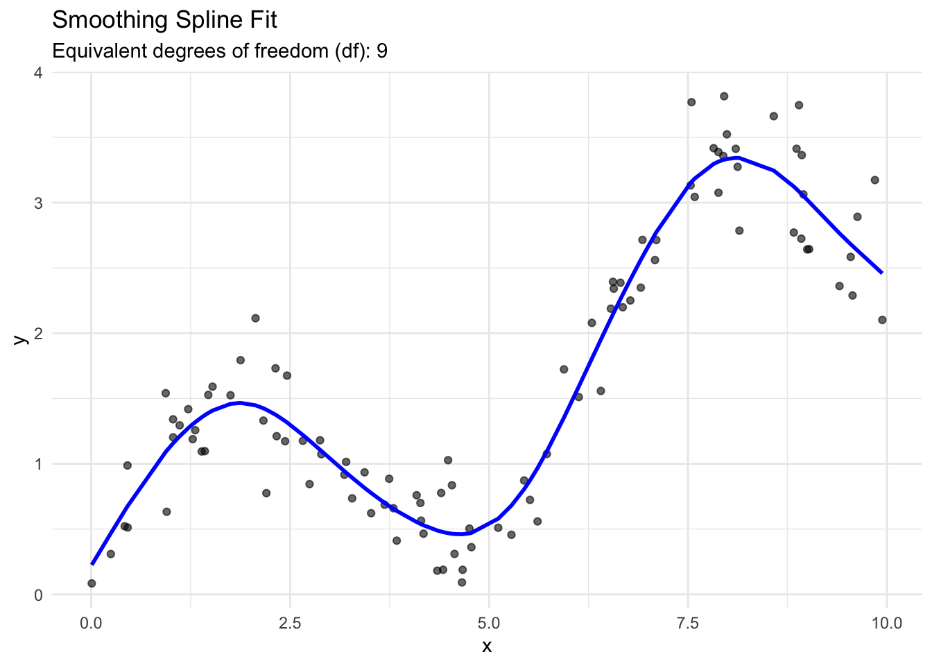

21.6 Controlling Smoothness

The key parameter in smoothing splines is the smoothing parameter (λ), which controls the trade-off between fit and smoothness. In R’s smooth.spline() function, this is controlled indirectly through the spar parameter or by specifying the degrees of freedom df:

# Fit smoothing splines with different degrees of freedom
spline_df3 <- smooth.spline(x, y, df = 3)    # Very smooth
spline_df8 <- smooth.spline(x, y, df = 8)    # Moderately smooth
spline_df15 <- smooth.spline(x, y, df = 15)  # Less smooth

# Create predictions for plotting
pred_data <- data.frame(
  x = x,
  df3 = predict(spline_df3, x)$y,
  df8 = predict(spline_df8, x)$y,
  df15 = predict(spline_df15, x)$y
)

# Plot comparison
ggplot(data, aes(x = x, y = y)) +
  geom_point(alpha = 0.4) +
  geom_line(data = pred_data, aes(y = df3, color = "df = 3"), linewidth = 1) +
  geom_line(data = pred_data, aes(y = df8, color = "df = 8"), linewidth = 1) +
  geom_line(data = pred_data, aes(y = df15, color = "df = 15"), linewidth = 1) +
  scale_color_manual(values = c("df = 3" = "blue", "df = 8" = "red", 
                               "df = 15" = "green")) +
  theme_minimal() +
  labs(title = "Smoothing Splines with Different Degrees of Freedom",
       color = "Smoothing Level")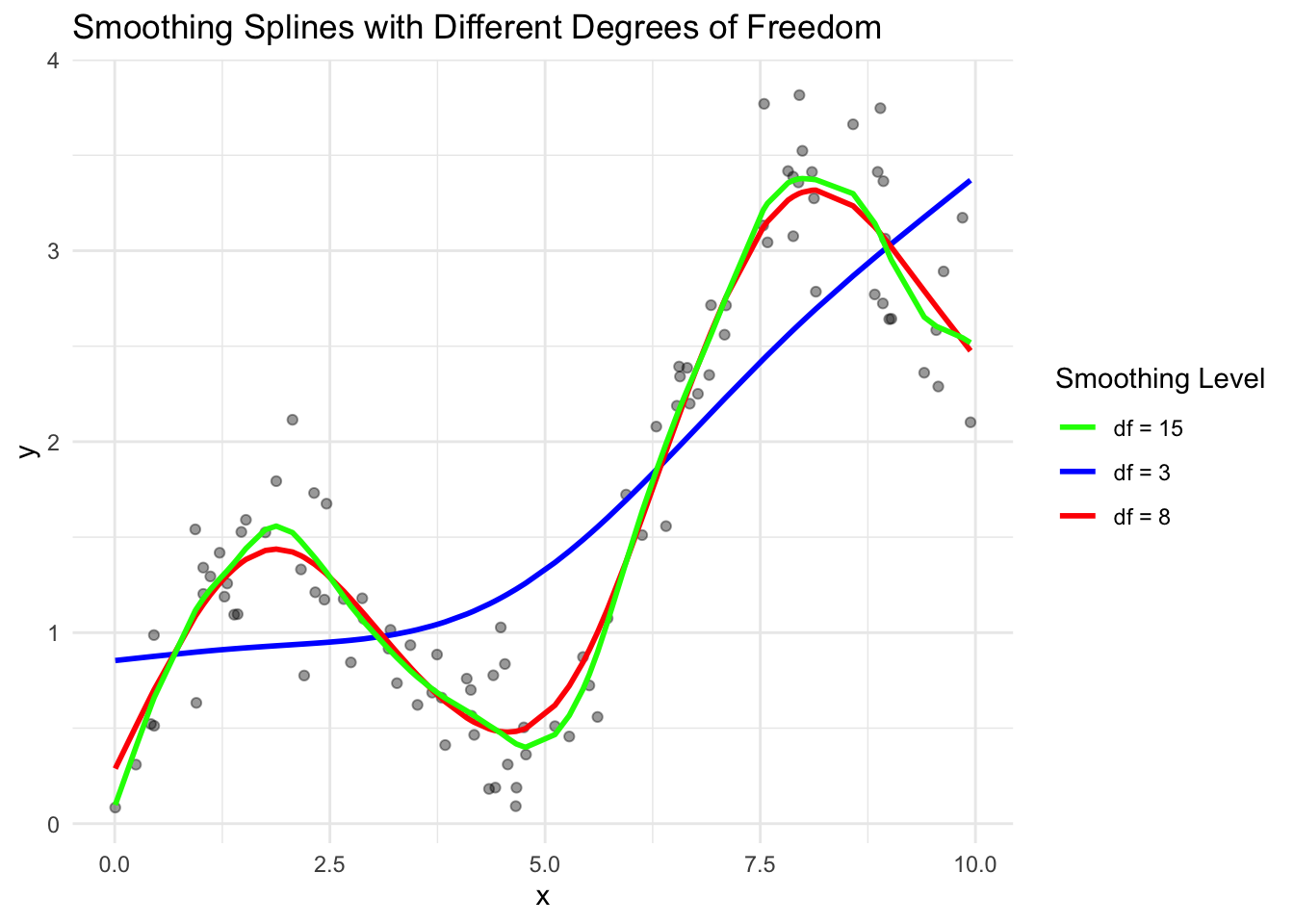

21.7 Cross-Validation for Optimal Smoothing

A key advantage of smoothing splines is the ability to select the optimal smoothing parameter using cross-validation:

# Fit smoothing spline with cross-validation
cv_spline <- smooth.spline(x, y, cv = TRUE)

# Plot CV-optimized spline
ggplot(data, aes(x = x, y = y)) +
  geom_point(alpha = 0.6) +
  geom_line(aes(y = predict(cv_spline, x)$y), 
            color = "purple", linewidth = 1) +
  theme_minimal() +
  labs(title = "Cross-Validated Smoothing Spline",
       subtitle = paste("Optimal df from CV:", round(cv_spline$df, 1)))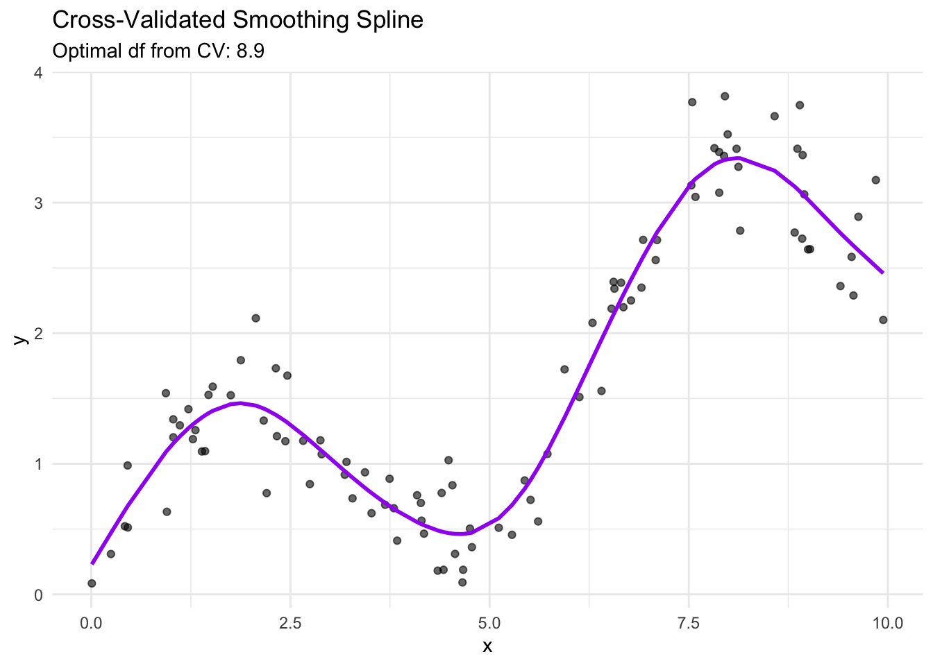

# Print summary info
cat("Cross-validation score:", cv_spline$cv.crit, "\n")

Cross-validation score: 0.09496418

cat("Equivalent degrees of freedom:", cv_spline$df, "\n")

Equivalent degrees of freedom: 8.917299

cat("Lambda:", format(cv_spline$lambda, scientific = TRUE), "\n")

Lambda: 3.828707e-04

21.8 Smoothing Splines in GAMs

Generalized Additive Models (GAMs) provide a more flexible framework for working with smoothing splines and other nonparametric components:

# Fit GAM with smoothing spline term
gam_model <- gam(y ~ s(x, bs = "cr"), data = data)

# Create a grid for smooth predictions
x_grid <- data.frame(x = seq(min(x), max(x), length = 200))
pred_gam <- predict(gam_model, x_grid, se.fit = TRUE)

# Add prediction intervals
x_grid$fit <- pred_gam$fit
x_grid$upper <- pred_gam$fit + 1.96 * pred_gam$se.fit
x_grid$lower <- pred_gam$fit - 1.96 * pred_gam$se.fit

# Plot GAM with confidence bands
ggplot() +
  geom_point(data = data, aes(x = x, y = y), alpha = 0.6) +
  geom_line(data = x_grid, aes(x = x, y = fit), 
            color = "blue", linewidth = 1) +
  geom_ribbon(data = x_grid, 
              aes(x = x, ymin = lower, ymax = upper),
              alpha = 0.2, fill = "blue") +
  theme_minimal() +
  labs(title = "Cubic Regression Spline from GAM",
       subtitle = "With 95% confidence bands")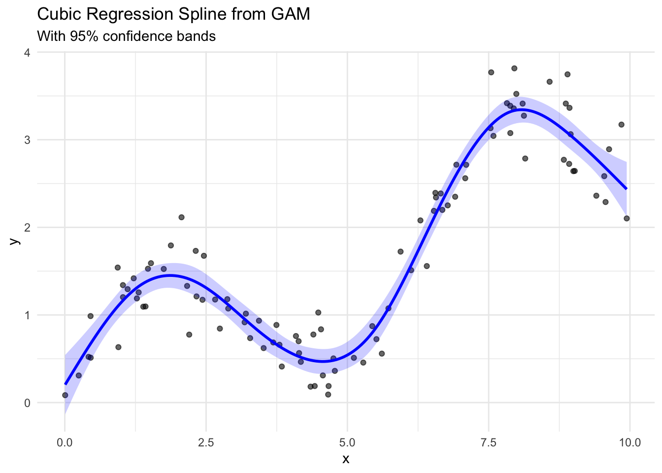

# Summary of the GAM
summary(gam_model)


Family: gaussian 
Link function: identity 

Formula:
y ~ s(x, bs = "cr")

Parametric coefficients:
            Estimate Std. Error t value Pr(>|t|)    
(Intercept)  1.67605    0.02911   57.58   <2e-16 ***
---
Signif. codes:  0 '***' 0.001 '**' 0.01 '*' 0.05 '.' 0.1 ' ' 1

Approximate significance of smooth terms:
       edf Ref.df   F p-value    
s(x) 7.166  8.214 150  <2e-16 ***
---
Signif. codes:  0 '***' 0.001 '**' 0.01 '*' 0.05 '.' 0.1 ' ' 1

R-sq.(adj) =  0.926   Deviance explained = 93.1%
GCV = 0.092257  Scale est. = 0.084724  n = 100

21.9 Real-World Example: Environmental Data

Let’s apply smoothing splines to analyze the relationship between ozone levels and temperature:

# Load and prepare the data
data(airquality)
aq_clean <- na.omit(airquality)

# Fit smoothing spline to ozone vs temperature
ozone_spline <- smooth.spline(aq_clean$Temp, aq_clean$Ozone, cv = TRUE)

# Fit GAM for comparison
ozone_gam <- gam(Ozone ~ s(Temp), data = aq_clean)

# Create prediction grid
temp_grid <- seq(min(aq_clean$Temp), max(aq_clean$Temp), length = 100)
spline_pred <- predict(ozone_spline, temp_grid)
gam_pred <- predict(ozone_gam, data.frame(Temp = temp_grid), se.fit = TRUE)

# Create prediction dataframe
pred_df <- data.frame(
  Temp = temp_grid,
  Spline = spline_pred$y,
  GAM = gam_pred$fit,
  GAM_lower = gam_pred$fit - 1.96 * gam_pred$se.fit,
  GAM_upper = gam_pred$fit + 1.96 * gam_pred$se.fit
)

# Plot results
ggplot() +
  geom_point(data = aq_clean, aes(x = Temp, y = Ozone), alpha = 0.6) +
  geom_line(data = pred_df, aes(x = Temp, y = Spline, color = "Smoothing Spline"), 
            linewidth = 1) +
  geom_line(data = pred_df, aes(x = Temp, y = GAM, color = "GAM"), 
            linewidth = 1) +
  geom_ribbon(data = pred_df, 
              aes(x = Temp, ymin = GAM_lower, ymax = GAM_upper),
              alpha = 0.2, fill = "red") +
  scale_color_manual(values = c("Smoothing Spline" = "blue", "GAM" = "red")) +
  theme_minimal() +
  labs(title = "Relationship Between Temperature and Ozone Levels",
       x = "Temperature (°F)",
       y = "Ozone (ppb)",
       color = "Method")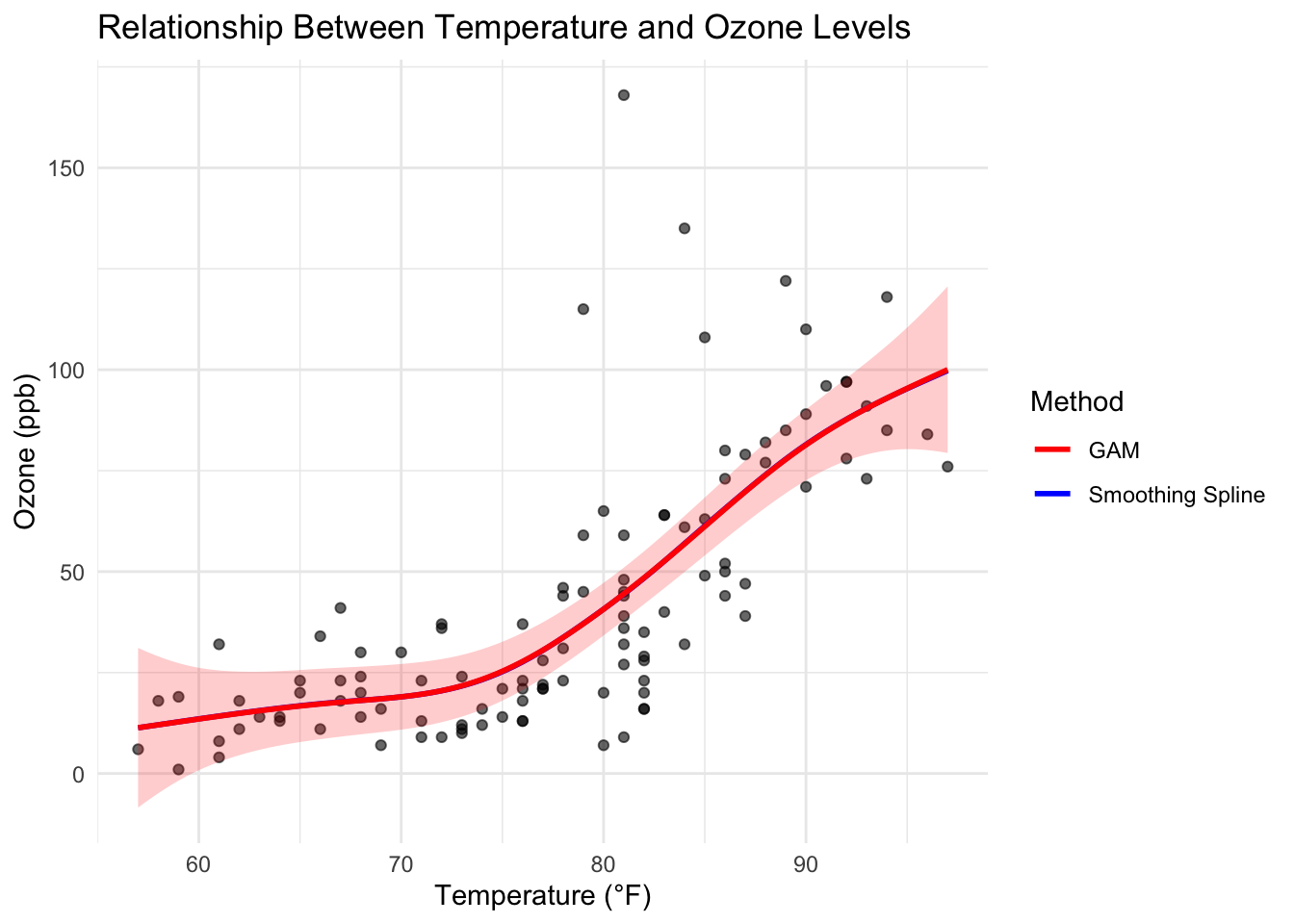

21.10 Conclusion

Smoothing splines provide a powerful and flexible approach to nonparametric regression. Key advantages include:

No need to specify a particular functional form
Ability to capture complex, non-linear relationships
Built-in methods for controlling smoothness via cross-validation
Interpretable results with confidence intervals (via GAMs)
Protection against overfitting

For more complex scenarios, consider: - Using GAMs to incorporate multiple predictors and different types of smoothers - Exploring tensor product smooths for interaction effects - Considering adaptive smoothing for varying complexity across the predictor range

21.11 References

Wood, S.N. (2017). Generalized Additive Models: An Introduction with R (2nd ed.). Chapman and Hall/CRC.
Hastie, T., & Tibshirani, R. (1990). Generalized Additive Models. Chapman and Hall/CRC.